If you’re looking for code to get started with our method, head to Getting Started With Some Code.
A Confound in the Data
We recently published new results indicating that there is a significant confound that must be controlled for when calculating similarity between neural networks: correlated, yet distinct features within individual data points. Examples of features like this are pretty straightforward and exist even at a conceptually high level: eyes and ears, wings and cockpits, tables and chairs. Really, any set of features that co-occur in inputs frequently and are correlated with the target class. To see why features like this are a problem let’s first look at the definition of the most widely used similarity metric, Linear Centered Kernel Alignment (Kornblith et al., 2019), or Linear CKA.
Linear Centered Kernel Alignment (CKA)
CKA computes a metric of similarity between two neural networks by comparing the neuron activations of each network on provided data points, usually taken from an iid test distribution. The process is simple: pass each data point through both networks and extract the activations at the layers you want to compare and stack these activations up into two matrices (one for each network). We consider the representation of an input point to be the activations recorded in a neural network at a specific layer of interest when the data point is fed through the network. We compute similarity by mean-centering the matrices along the columns, and computing the following function:
This will provide you with a score in the range , with higher values indicating more similar networks. What we see in the equation above, effectively, is that CKA is computing a normalized measure of the covariance between neurons across networks. Likewise, all other existing metrics for network similarity use some form of (potentially nonlinear) feature correlation.
Linear CKA is easily translated into a few lines of PyTorch:
| |
Idealized Neurons
With the idea of feature correlation in mind let’s picture two networks, each having an idealized neuron. The first network has a
cat-ear detector neuron–it fires when there are cat ears present in the image and does not otherwise. The other network has a neuron that is quite similar, but this one is a
cat-tail detector‚ which only fires when cat tails are found. These features are distinct both visually and conceptually, but their neurons will show high correlation: images containing cat tails are very likely to contain cat ears, and conversely when cat ears are not present there are likely to be no cat tails. CKA will find these networks to be quite similar, despite their reliance on entirely different features.
Overcoming the Confound
We need a way to isolate the features in an image used by a network while randomizing or discarding all others (i.e., preserve the
cat-tail in an image of a cat, while randomizing / discarding every other feature, including the
cat-ears).
A technique known as Representation Inversion can do exactly this. Representation inversion was introduced by Ilyas et al. (2019) as a way to understand the features learned by robust and non-robust networks. This method constructs model-specific datasets in which all features not used by a classifier are randomized, thus removing co-occurring features that are not utilized by the model being used to produce the inversions.
Given a classification dataset, we randomly choose pairs of inputs that have different labels. The first of each pair will be the seed image s and the second the target image t. Using the seed image as a starting point, we perform gradient descent to find an image that induces the same activations at the representation layer, , as the target image1. The fact that we are performing a local search is critical here, because there are many possible inverse images that match the activations. We construct this image through gradient descent in input space by optimizing the following objective:
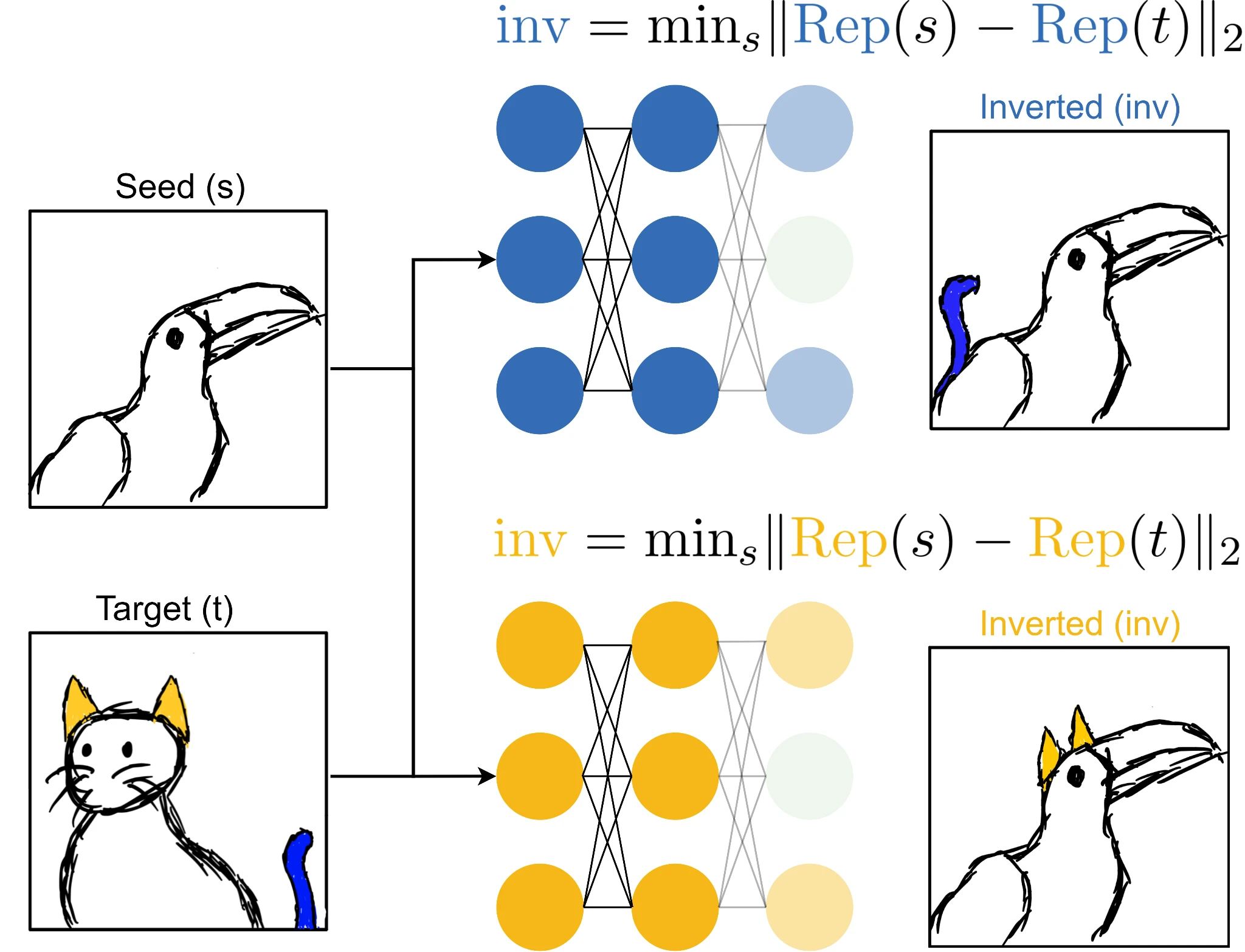
By sampling pairs of seed and target images that have distinct labels we eliminate features correlated with the target class that are not used by the model for classification of the target class. This is illustrated below for our two idealized
cat-tail and
cat-ear classifiers:

Here, our seed image is a toucan and our target image is a cat. Representation inversion through our
cat-tail network will produce an inverted image retaining the pertinent features of the target image while ignoring all other irrelevant features, resulting in a toucan with a cat tail. This happens because adding
cat-ear features into our seed image will not move the representation of the seed image closer to the target as the network utilizes only
cat-tails for classification of cats.
When our cat tail toucan is fed through both networks, we will find that while our
cat-tail neuron stays active, our
cat-ear neuron never fires as this feature isn’t present! We’ve successfully isolated the features of the blue network in our target image and now can calculate similarity more accurately. The above figure also illustrates this process for the
cat-ear network, however, representation inversion under this network produces a toucan with ears rather than a tail.
By repeating this process on many pairs of images sampled from a dataset we can produce a new inverted dataset wherein each image contains only the relevant features for the model while all others have been randomized. Calculating similarity between our inverting-model and an arbitrary network using the inverted dataset should now give us a much more accurate estimation of their similarity 2.
Results

Above we present two heatmaps showing CKA similarity calculated across pairs of 9 architectures trained on ImageNet. The left heatmap shows similarity on a set of images taken from the ImageNet validation set, as is normally done. Across the board we see that similarity is quite high between any pair of architectures, averaging at . On the right we calculate similarity between the same set of architectures, however each row and column pair is evaluated using the row model’s inverted dataset. Here we see that similarity is actually quite low when we isolate the features used by models!
Alongside these results we investigated how robust training affects the similarity of architectures under our proposed metric and multiple others. Surprisingly, we found that as the robustness of an architecture increases so too does its similarity to every other architecture, at any level of robustness. If you’re interested in learning more, we invite you to give the paper a read.
Getting Started With Some Code
If you’d like to give this method a shot with your own models and datasets, we provide some code to get you started using PyTorch and the Robustness library. This code expects your model to be an AttackerModel provided by the Robustness library‚ for custom architectures check the documentation here to see how to convert your model to one, it’s not too hard.
All you need to do is provide the function invert_images with a model (AttackerModel), a batched set of seed images, and a batched set of target images (one for each seed image)–all other hyperparameters default to the values used in our paper.
Before you start there are a couple things to double check:
- Make sure that your seed and target pairs are from different classes.
- Make sure that your models are in evaluation mode.
| |
Conclusions
While I mainly focused on our proposed metric in this article, I briefly wanted to discuss some of the interesting takeaways we included in the paper. The fact that robustness systematically increases a model’s similarity to any arbitrary other model, regardless of architecture or initialization, is a significant one. Within the representation learning community, some researchers have posed a universality hypothesis. This hypothesis conjectures that the features networks learn from their data are universal‚ in that they are shared across distinct initializations or architectures. Our results imply a modified universality hypothesis, suggesting that under sufficient constraints (i.e., a robustness constraint), diverse architectures will converge on a similar set of learned features. This could mean that empirical analysis of a single robust neural network can reveal insight into every other neural network–possibly bringing us closer to understanding the nature of adversarial robustness itself. This is especially exciting in light of research looking at similarities between the representations learned by neural networks and brains.
References
[1] Haydn T. Jones, Jacob M. Springer, Garrett T. Kenyon, and Juston S. Moore. “If You’ve Trained One You’ve Trained Them All: Inter-Architecture Similarity Increases With Robustness.” UAI (2022).
[2] Simon Kornblith, Mohammad Norouzi, Honglak Lee, and Geoffrey E. Hinton. “Similarity of Neural Network Representations Revisited.” ICML (2019).
[3] Andrew Ilyas, Shibani Santurkar, Dimitris Tsipras, Logan Engstrom, Brandon Tran, and Aleksander Madry. “Adversarial Examples Are Not Bugs, They are Features.” NeurIPS (2019).
[4] Vedant Nanda, Till Speicher, Camila Kolling, John P. Dickerson, Krishna Gummadi, and Adrian Weller. “Measuring Representational Robustness of Neural Networks Through Shared Invariances.” ICML (2022).
LA-UR-22-27916
We define the representation layer to be the layer before the fully connected output layer. We are most interested in this layer as it should have the richest representation of the input image. ↩︎
It turns out that our metric of network similarity was simultaneously proposed and published by Nanda et al. in “Measuring Representational Robustness of Neural Networks Through Shared Invariances”, where they call this metric “STIR”. ↩︎